latent_series_LTP_UCS=as.factor(viterbi(hmm_init_LTP_UCS,obsWood))
latent_series_LTP_CS=as.factor(viterbi(hmm_init_LTP_CS,obsWood))
latent_series_HTP_UCS=as.factor(viterbi(hmm_init_HTP_UCS,obsWood))
latent_series_HTP_CS=as.factor(viterbi(hmm_init_HTP_CS,obsWood))
list_latent_series=list(latent_series_LTP_UCS,
                        latent_series_LTP_CS,
                        latent_series_HTP_UCS,
latent_series_HTP_CS)3 Predicting hidden states
3.1 The Viterbi algorithm
The Viterbi algorithm is a dynamic programming algorithm for finding the most likely sequence of hidden states – called the Viterbi path – that results in a sequence of observed events, especially in the context of Markov information sources and hidden Markov models.
The most likely series of states \(s_1,\dots,s_n\) underlying the observations is found recursively.
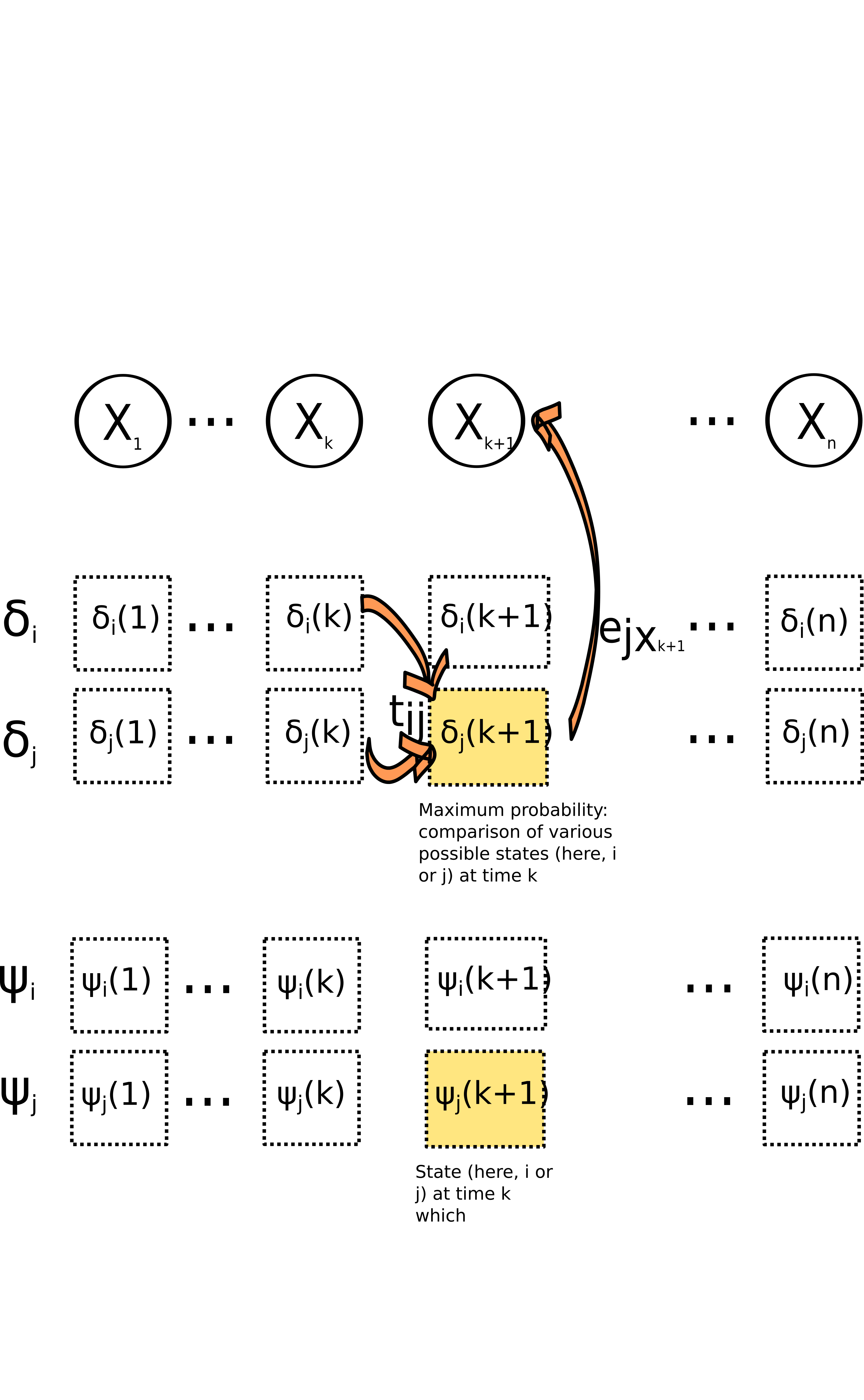
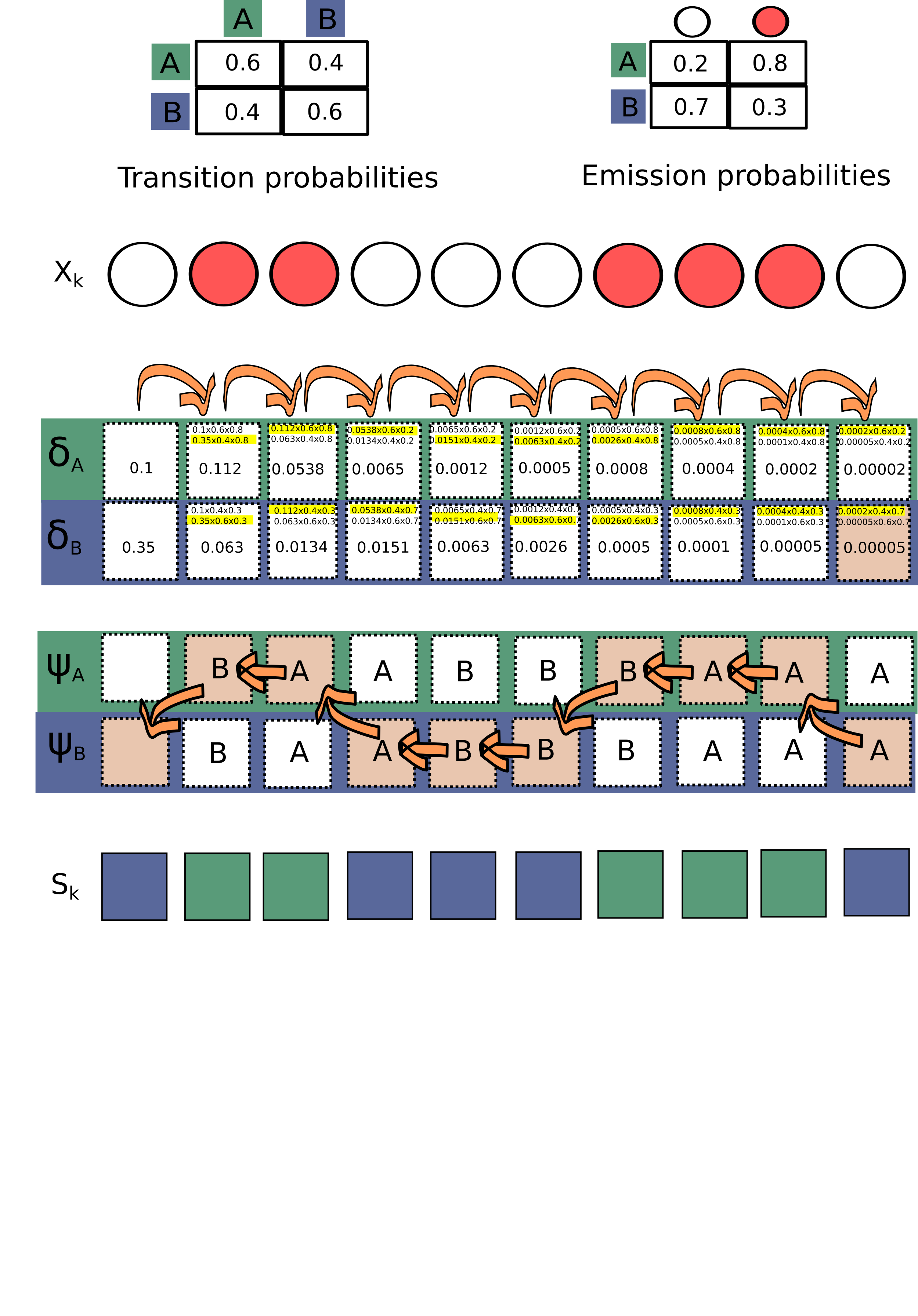
Let us define \(\delta_i(k)\) as the highest probability of observations \(X_1,X_2,....,X_k\) considering all possible paths (\(S_1=s_1,S_2=s_2,\ldots, S_k=i\)), (i.e. all possible paths going from step 1 to \(k\), and ending with state \(i\)):
\[ \delta_i(k) = max_{s_1,s_2,....s_{k-1}}pr(X_1,X_2,\ldots,X_k,S_1=s_1,S_2=s_2,\ldots,S_k=i)/\theta) \]
We note \(\phi_i(k)\) the argument of this maximum, i.e.
\[ \phi_i(k) = Argmax_{s_1,s_2,....s_{k-1}}pr(X_1,X_2,\ldots,X_k,S_1=s_1,S_2=s_2,\ldots,S_k=i)/\theta) \]
Hence, \(\delta_i(k)\) corresponds to a maximum probability while \(\phi_i(k)\) corresponds to the state \(i\) that maximizes it.
\(\delta_j(k+1)\) can be expressed as a function of \(\delta_i(k)\):
\[ \delta_j(k+1) = [max_i\delta_i(k)t_{ij}]*e_{jx_k+1} \]
Starting with
\[ \delta_1(i)=\pi_ie_{ix_1} \]
we can thus calculate recursively \(\delta_i(k)\) and \(\phi_i(k)\) for all possible states \(i\), as it is illustrated in figure \(\ref{Viterbi}\).
3.2 Applying the Viterbi aligorithm in practice
Now we calculate the latent series according to the four different sets of initial parameters. We do not calculate them using the fitted HMMs because they are very close to each other and we want to show the effect of parameters on the inferred states sequence.
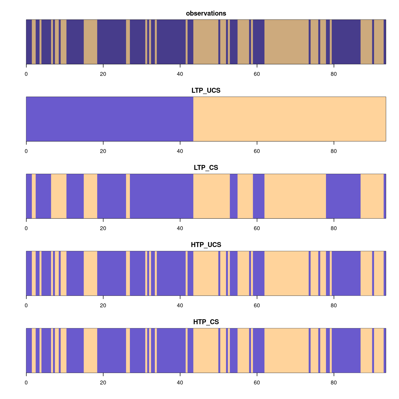
Unsurprisingly, when transition probabilities are higher (HTP_* vs LTP_*), the segments tend to be shorter. The emission probabilities also have an effect on the segments’ lengths: contrasted states (in the case LTP_CS vs LTP_UCS) hence correspond to shorter segments.