Let’s consider a qualitative geomorphological descriptor a river. This indicator has been built through a hierarchical clustering analysis based on several quantitative variables, namely:
f.slope: log(slope)
f.sinuosity: log(sinuosity -1)
f.vall_bott_W: log(valley bottom width)
f.wat_cov: logit(area under water divided by area of the active channel)
f.act_chan_cov: log(area of the active channel divided by catchment area)
f.act_chan_vW: log(interquartile range of active channel width)
The individuals are homogeneous reaches of average length 1.7km.
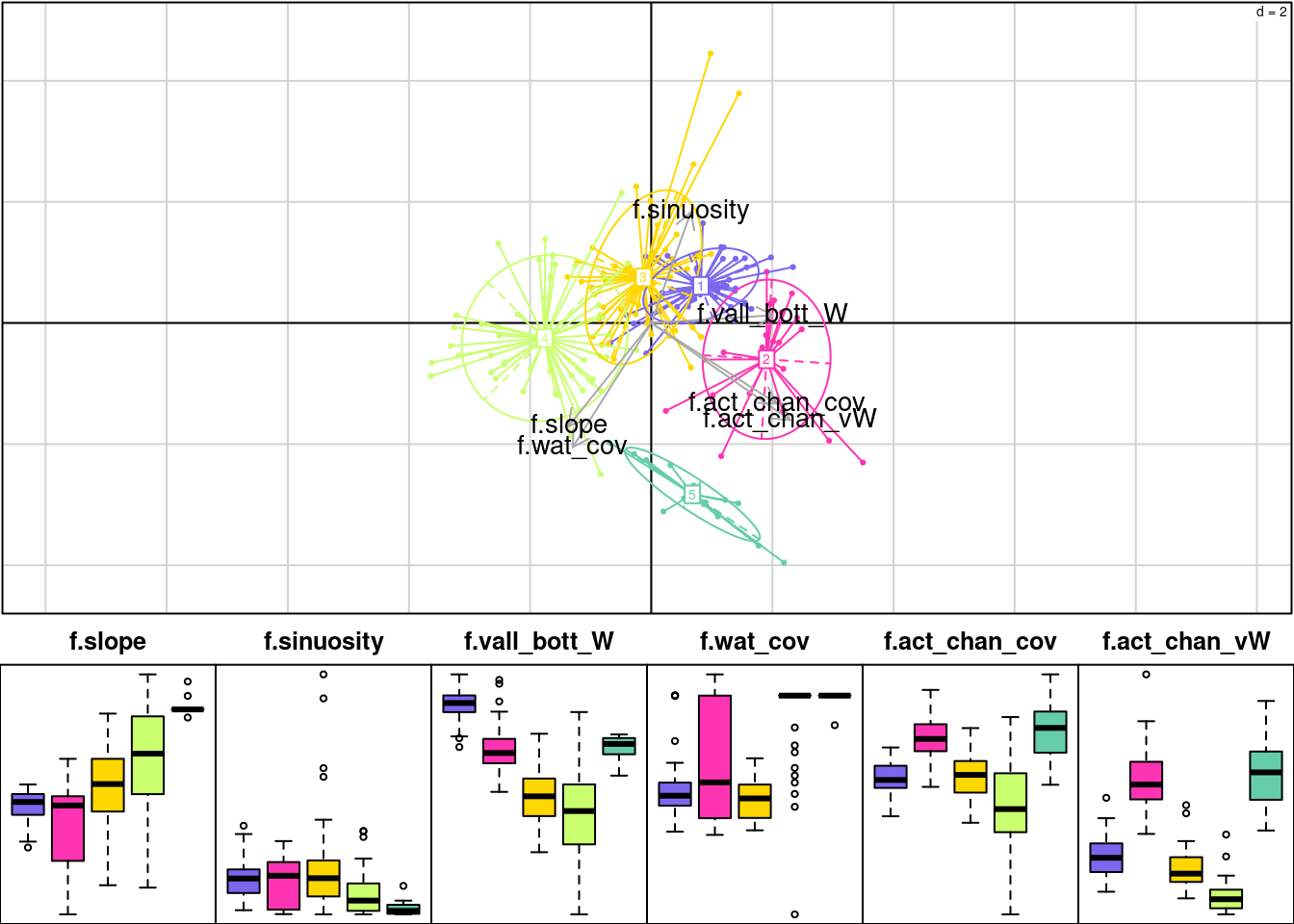
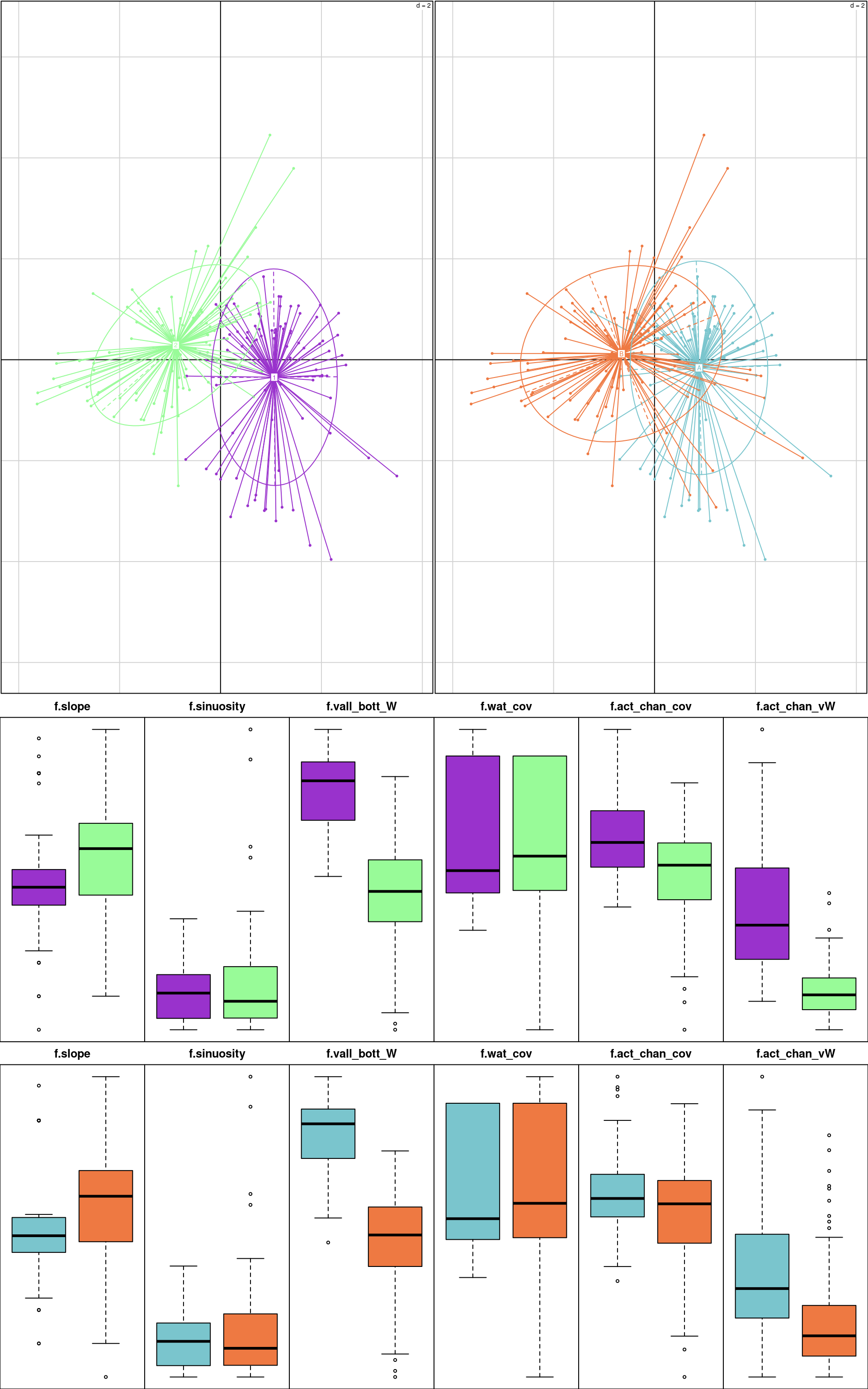
Figure 4.1: Description of classes. A Principal Component Analysis has been performed to help with the description.
Figure Figure 4.1 shows the quantitative geomorphological features of the 5 classes defined through hierarchical clustering.
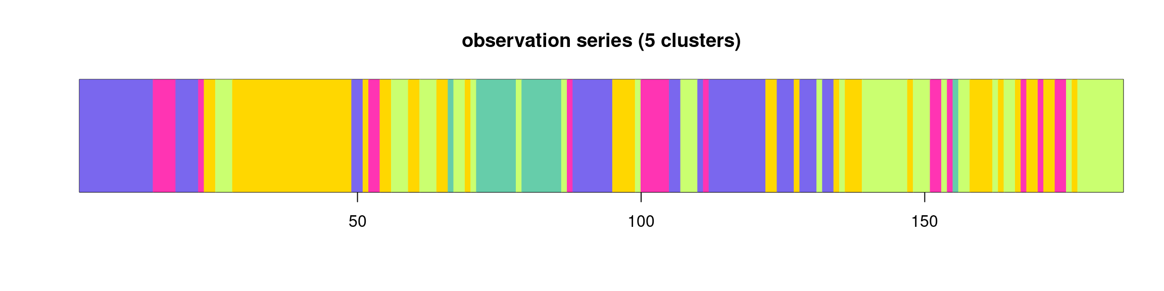
Figure 4.2: Description of classes
Figure Figure 4.2 displays the sequence of classes along the river.
4.1.2 Fit of a HMM
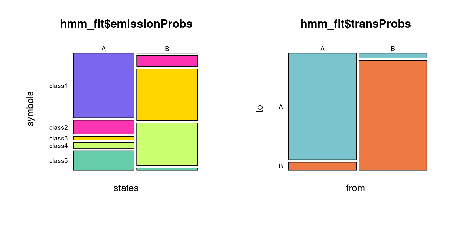
We hypothesize that there are actually two hidden states (let’s call them “A” and “B”) behind the observed sequence of series). The proportions of classes in the observation series is:
      symbols
states class1 class2 class3 class4 class5
     A    0.6   0.13   0.03   0.06   0.18
     B    0.0   0.10   0.48   0.40   0.02
round(hmm_fit$transProbs,2)
    to
from    A    B
   A 0.93 0.07
   B 0.04 0.96
Figure Figure 4.3 illustrates the differences between states A and B: A is characterized by a frequent occurence of classes 3 and 4 while B is characterized by a frequent occurence of classes 1, 2 and 5.
Now, we use the fitted HMM to infer the hidden states series:
seriesHMM=as.factor(viterbi(hmm_fit,series5))
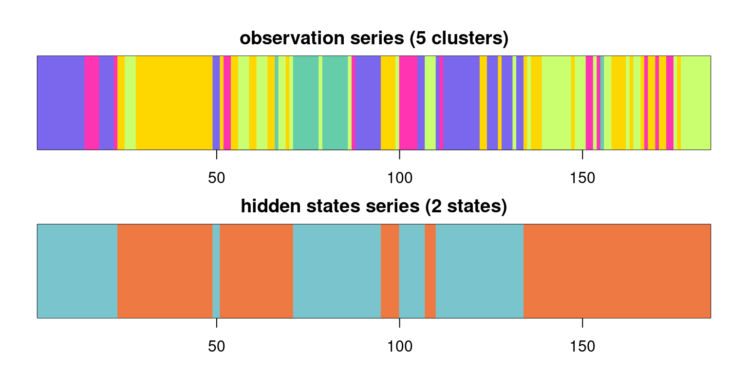
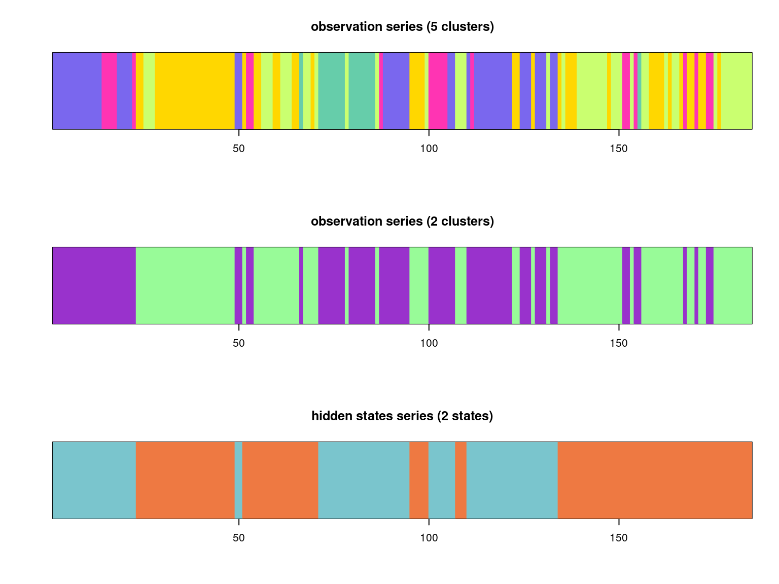
Figure 4.4: 1) observation series (classification into 5 clusters based on quantitative variables) 2) hidden states series (classification into two states based on observation series consisting of 5 possible clusters).
Figure Figure 4.4 displays the observation and estimated states series.
4.1.3 Discussion: HMM segmentation vs clustering
A HMM is primarily designed to describe the sequence of hidden states underlying the observation of a series. Doing so, it cuts a qualitative signal into homogeneous segments.
In this example, the data at hand has been used to first define 5 classes, and then a HMM model has been carried out to define 2 states based on these 5 classes. One can wonder why not define 2 classes directly.
Actually, these two methods, although they seemingly result in the same kind of output (i.e. a 2-classes segmentation of the river) do not proceed according to the same principles.
Hierarchical clustering makes no direct use in the geographical information in the data. The fact that two successive reaches fall into the same class is only due to the fact that two reaches tend to have similar geomorphological descriptions when they are close to each other.
On the other hand, a HMM model uses both geomorphological descriptors AND geographical information (i.e. the location of reaches in the sequence) to define which state they are most likely to result from.
To illustrate this we will use the quantitative data at hand to define a 2-classes description based on a hierarchical clustering. Figure Figure 4.5 shows the characteristics of these 2 classes as well as the characteristics of reaches occurring presumably in states A and B.
Figure 4.5: Comparison of 1) classes (output of hierarchical clustering with 2 classes) and 2) hidden states as estimated based on a HMM model.
Figure Figure 4.5 illustrates the closeness (in terms of descriptors) of classes either inferred (based on several quantitative variables) through hierarchical clustering and states based on a 5-classes descriptor as defined through a HMM model fit.
On the other hand, figure Figure 4.6 shows that there are some differences between segments either defined as the projection of the 2-classes categorization along the river (for hierarchical clustering) or defined as the most probable states path (for HMM). Taking into account the geographical succession of reaches and not only geomorphological features, the HMM path provides a less fragmented segmentation.
Figure 4.6: Comparison of 1) observation series (classification into 5 clusters based on quantitative variables) 2) observation series (classification into 2 clusters based on quantitative variables) 3) hidden states series (classification into two states based on observation series consisting of 5 possible clusters).
4.2 Textual analysis example
Let’s consider an extract of a Sherlock Holmes novel.
We are interested in distinguishing the parts where the focus is mainly on Sherlock Holmes, to parts where the attention is mainly focused on the narrator, Dr Watson. We want to do this on all Sherlock Holmes novels so that this distinction should be done automatically (though here we will only use a short extract as an example).
We categorize words into 3 categories:
a neutral category (outcome “blah”)
a Sherlock Holmes-centered category (outome “he”)
a John Watson-centered category (outcome “I”)
           text observations
1            To         blah
2      Sherlock           he
3        Holmes           he
4           she         blah
5            is         blah
6        always         blah
7           the         blah
8         woman         blah
9             .         blah
10            I            I
11         have         blah
12       seldom         blah
13        heard         blah
14          him           he
15      mention         blah
16          her         blah
17        under         blah
18          any         blah
19        other         blah
20         name         blah
21            .         blah
22           In         blah
23          his           he
24         eyes         blah
25          she         blah
26     eclipses         blah
27          and         blah
28 predominates         blah
29          the         blah
30        whole         blah
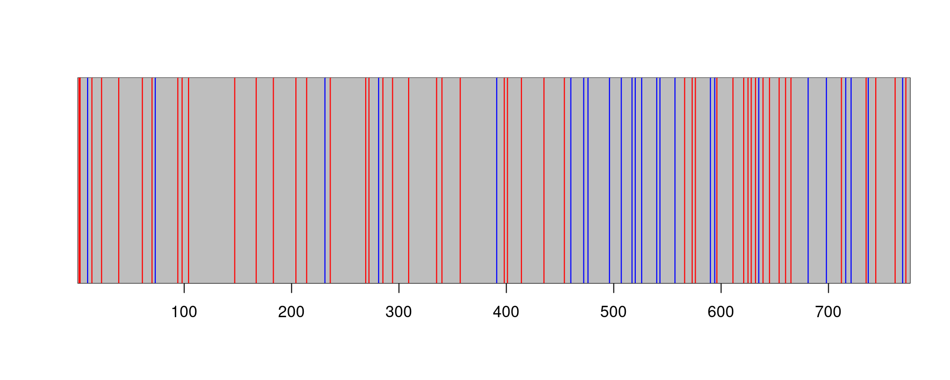
Figure Figure 4.7 shows how the sequence of outcomes looks like for our example.
Figure 4.7: The observation series: each point corresponds to a word in a text. Blue points correspond to an occurrence of an ‘I’ outcome, while red points correspond to an occurrence of a ‘he’ outcome.
observations
      blah         he          I
0.90592784 0.06185567 0.03221649
myprop=as.vector(myprop)
We initialize the emission matrix stating that occurrence of the “he” outcome should be more frequent in the Holmes-centered parts while the “I” will be more frequent in the Watson-centered parts.
        symbols
states   blah   he    I
  Holmes 0.91 0.07 0.02
  Watson 0.90 0.00 0.10
print(round(hmm_fit$transProbs,2))
        to
from     Holmes Watson
  Holmes   1.00   0.00
  Watson   0.01   0.99
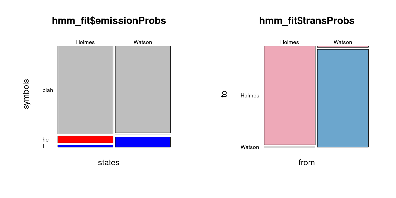
The characteristics of states “Holmes” and “Watson” are displayed in figure Figure 4.8. Watson (outcome “I”), as a narrator, never completely disappears from the text even in Holmes-centered parts, while Watson-parts are characterized by a null occurrence of outcome “he”.
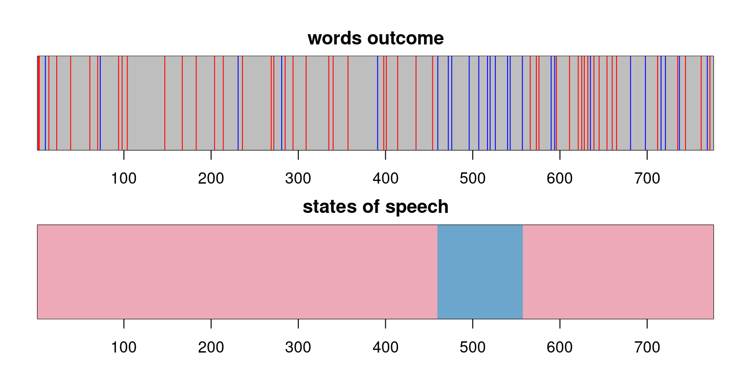
Figure 4.8: Fitted parameters of the HMM.
Now, we use the fitted HMM to infer the hidden states series:
Figure Figure 4.9 displays the observation and estimated states series. There is only one part of the text which appears to be Watson-centered (according to how Watson-centerization is defined, i.e. total disappearance of “he” outcomes.)