5  Continuous Hidden Markov Models

Although states in Hidden Markov Models are by definition categorical, the observations might be quantitative rather than categorical. In these cases the HMM might be called continuous observations HMMs or continuous HMMs (though the quantitative outputs might actually have discrete or pseudo-continous distributions).

We will illustrate such a model in the case of a Poisson distribution. To do so we will consider an observed series consisting of the number of wood rafts observed along a river.

To fit the Poisson Hidden Markov Model we use R scripts provided as an annex to the book Zucchini and MacDonald (2009) and provided in the current repo under scripts:

source("scripts/scripts_Zucchini_and_McDonald_2009.R")

# number of wood rafts
woodrafts= readr::read_csv("data/wood_abundance.csv")
pk=woodrafts$PK
x=woodrafts$nbre_embacle

ggplot(woodrafts, aes(x=pk, y=nbre_embacle))+
  geom_path()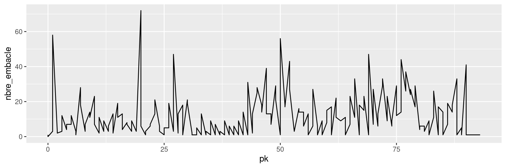

An example of observation series: occurrence of wood 500 meter-long sections of the river.

5.1 Initial parameters

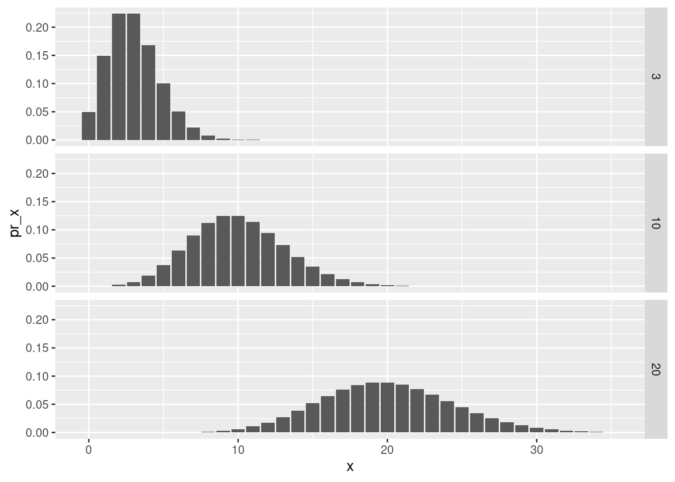
We will initialize a HMM with three states, corresponding to a distribution of wood rafts with an average outcome that is:

• low (\(\lambda\)=3)

• medium (\(\lambda\)=10)

• high (\(\lambda\)=20)

lambda0=c(3,10,20)

The corresponding distributions look like this:

Now, let’s initialize the transition matrix (with 3 rows and 3 columns since we consider three possible states). We make it such that the transition from one state to another is rather low (5% total):

gamma0=matrix(rep(0.025,9),nrow=3)
diag(gamma0)=0.95
gamma0

      [,1]  [,2]  [,3]
[1,] 0.950 0.025 0.025
[2,] 0.025 0.950 0.025
[3,] 0.025 0.025 0.950

We now have defined all necessary parameters:

parvect=pois.HMM.pn2pw(m=3,lambda=lambda0,gamma=gamma0)

5.2 Fitting the model

Now, let us fit the model through maximum likelihood estimation:

fitted_HMM_ML=pois.HMM.mle(x,m=3,lambda0,gamma0)

fitted_HMM_ML

$lambda
[1]  2.585161 12.725351 34.177599

$gamma
          [,1]      [,2]      [,3]
[1,] 0.4795649 0.4044502 0.1159850
[2,] 0.3936670 0.4105721 0.1957609
[3,] 0.4205519 0.3577776 0.2216705

$delta
[1] 0.4355214 0.3991789 0.1652996

$code
NULL

$mllk
[1] 691.3476

$AIC
[1] 1400.695

$BIC
[1] 1429.823

woodrafts <- woodrafts %>% 
  mutate(xsim=pois.HMM.generate_sample(n=n(),
                                       m=3,
                                       lambda=fitted_HMM_ML$lambda,
                                       gamma=fitted_HMM_ML$gamma))
ggplot(woodrafts, aes(x=pk, y=xsim))+
  geom_path()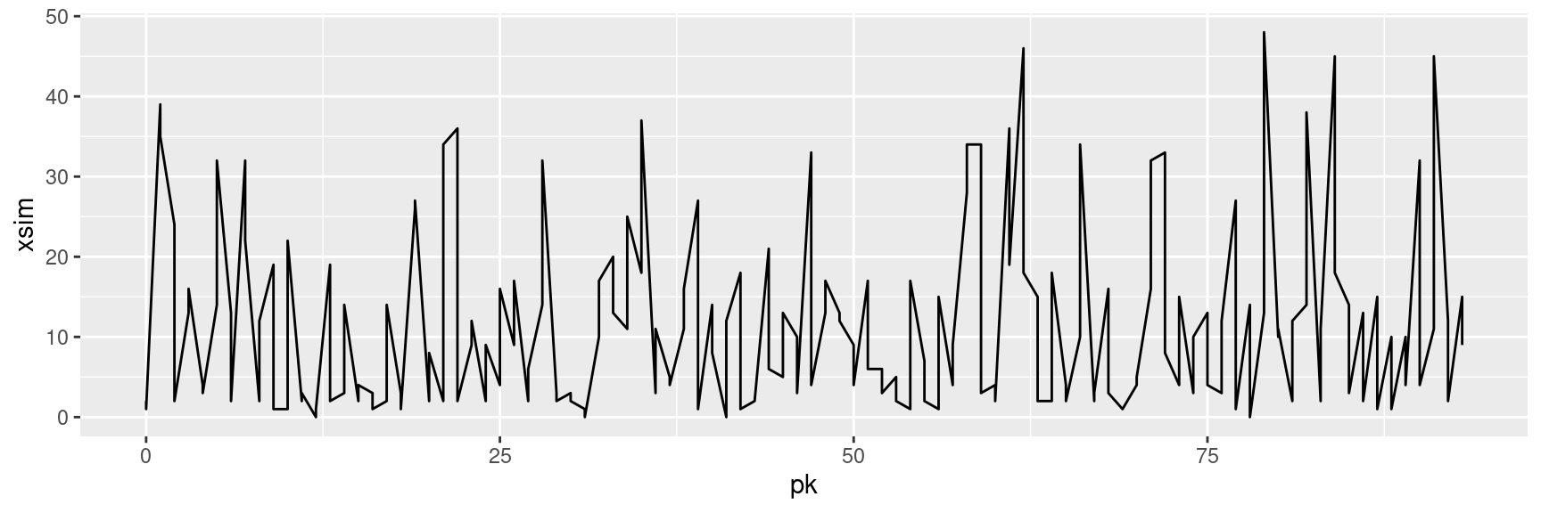

An example of simulated series: possible occurrence of wood rafts according to fitted model.

Other methods for fitting a model exist:

fitted_HMM_EM=pois.HMM.EM(x,m=3,fitted_HMM_ML$lambda,fitted_HMM_ML$gamma, delta=NULL)
fitted_HMM_EM

$lambda
[1]  2.554198 12.650083 34.117710

$gamma
          [,1]      [,2]      [,3]
[1,] 0.4713464 0.4115508 0.1171027
[2,] 0.3895688 0.4127975 0.1976337
[3,] 0.4128963 0.3641187 0.2229850

$delta
[1] 1 0 0

$mllk
[1] 690.5085

$AIC
[1] 1403.017

$BIC
[1] 1438.618

We can now associate the states with the estimates of mean outcome \(\hat\lambda_i\):

tib_states=tibble::tibble(states=1:3,
                          lambda_est=fitted_HMM_EM$lambda)
tib_states

# A tibble: 3 × 2
  states lambda_est
   <int>      <dbl>
1      1       2.55
2      2      12.7 
3      3      34.1 

woodrafts <- woodrafts %>% 
  mutate(states=pois.HMM.viterbi(x,
                                 m=3,
                                 lambda=fitted_HMM_EM$lambda,
                                 fitted_HMM_EM$gamma,
                                 delta=NULL)) %>% 
  left_join(tib_states,by=c("states"))
head(woodrafts)

# A tibble: 6 × 5
     PK nbre_embacle  xsim states lambda_est
  <dbl>        <dbl> <int>  <dbl>      <dbl>
1     0            1     2      1       2.55
2     0            0     1      1       2.55
3     1            3    39      1       2.55
4     1           58    35      3      34.1 
5     2            3    24      1       2.55
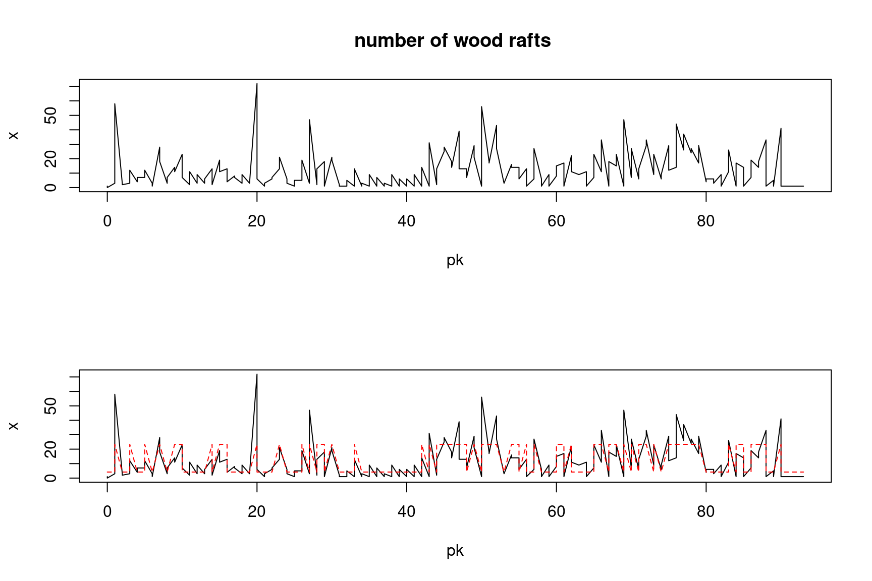
6     2            2     2      1       2.55

#|fig-cap: "Series of observed data (plain black line) and estimated hidden states (red dotted line)"
ggplot(woodrafts, aes(x=pk,y=nbre_embacle))+
  geom_path()+
  geom_line(aes(y=lambda_est), col="red",linetype=3)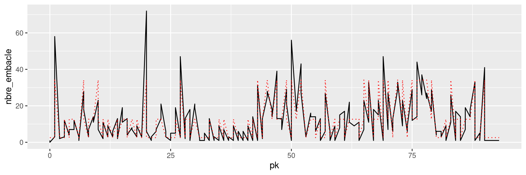

5.3 Considering two states

m=2
lambda0=c(10,80)
gamma0=matrix(rep(0.025,m^2),nrow=m)
diag(gamma0)=0.95
parvect=pois.HMM.pn2pw(m=m,lambda=lambda0,gamma=gamma0)
fitted.HMM=pois.HMM.mle(x,m=m,lambda0,gamma0)

Warning in nlm(pois.HMM.mllk, parvect0, x = x, m = m): NA / Inf remplacé par la
valeur maximale positive

print(fitted.HMM)

$lambda
[1]  4.186209 23.368149

$gamma
          [,1]      [,2]
[1,] 0.6841098 0.3158902
[2,] 0.4752263 0.5247737

$delta
[1] 0.6007033 0.3992967

$code
NULL

$mllk
[1] 807.4495

$AIC
[1] 1622.899

$BIC
[1] 1635.845

fitted.HMM.EM=pois.HMM.EM(x,m=m,fitted.HMM$lambda,fitted.HMM$gamma, delta=NULL)

states=pois.HMM.viterbi(x,m=m,lambda=fitted.HMM.EM$lambda,fitted.HMM.EM$gamma,delta=NULL)
print(states)

  [1] 1 1 1 2 1 1 1 2 1 1 1 2 1 1 2 2 1 1 2 2 2 1 1 1 1 1 1 1 2 1 2 2 2 1 1 1 1
 [38] 1 1 1 2 1 1 1 1 1 2 2 1 1 1 1 1 2 1 2 1 2 2 1 2 2 1 1 1 1 1 2 1 1 1 1 1 1
 [75] 1 1 1 1 1 1 1 1 1 1 1 2 1 2 1 2 2 2 2 2 2 2 2 1 2 2 1 2 2 2 2 2 1 1 2 2 2
[112] 1 2 1 1 2 1 1 1 1 1 2 2 1 2 1 1 1 1 1 1 2 2 2 1 2 2 2 1 2 1 2 1 2 2 2 1 2
[149] 1 1 2 2 2 2 2 2 2 2 2 2 1 1 1 1 1 1 1 2 1 2 2 1 1 2 2 2 2 1 1 1 2 1 1 1 1
[186] 1 1 1

layout(matrix(1:2, nrow=2))
plot(pk,x,type="l", main="number of wood rafts ")
plot(pk,x, type="l")
points(pk,fitted.HMM.EM$lambda[states], col="red", type="l", lty=2)

Zucchini, W., and I. L. MacDonald. 2009. Hidden Markov Models for Time Series: An Introduction Using r, 1st Edition. Chapman & Hall/CRC Monographs on St,atistics and Applied Probability. CRC Press. https://doi.org/https://doi.org/10.1201/9781420010893.