Produce and display basic bibliometrics

library(bibou)
library(bibliometrix)
library(tidyverse)

Table tib_doc

The table produced by bib_tib_doc() is structured as one row = one document.

tib_doc=bib_tib_doc("data/savedrecs_clean.bib")
#> 
#> Converting your isi collection into a bibliographic dataframe
#> 
#> Done!
#> 
#> 
#> Generating affiliation field tag AU_UN from C1:  Done!

Based on this table we can produce a variety of tabular and graphical results using tidy tools (especially dplyr and ggplot2). For instance, we can study the number of documents per publication year, or type, or source.

Example: number of documents per publication year

tib=tib_doc %>% 
  mutate(ntot=n()) %>% 
  group_by(PY,ntot) %>% 
  summarise(n=n(),.groups="drop") %>% 
  mutate(prop=n/ntot)
ggplot(tib, aes(x=PY, y = prop))+
  geom_col()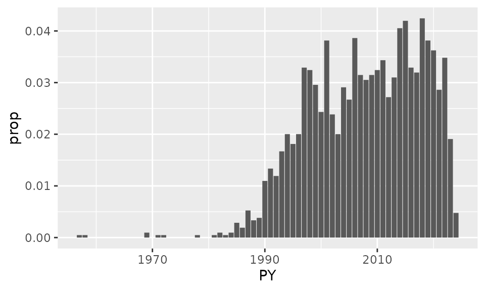

Example: number of documents per publication year and source

Here, we will show the number of publications per year and per journal (showing only journals that account for a total of more than 25 documents).

tib=tib_doc %>% 
  group_by(SO) %>% 
  mutate(ntot=n()) %>% 
  group_by(PY,SO,ntot) %>% 
  summarise(n=n(),.groups="drop") %>% 
  mutate(prop=n/ntot) %>% 
  filter(ntot>=50)
ggplot(tib, aes(x=PY, y = prop,fill=SO))+
  geom_col()+
  facet_wrap(facets=vars(SO),ncol=1)+
  theme(legend.position="none")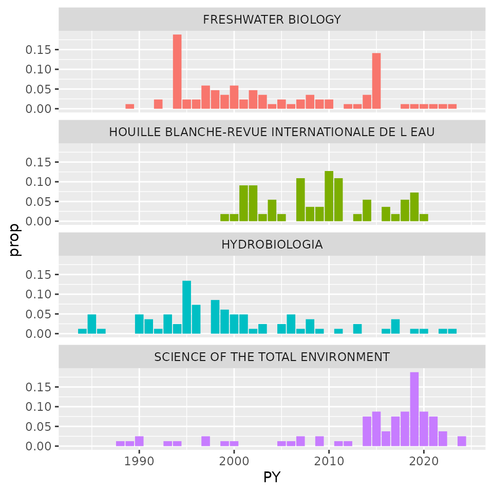

Table tib_doc_author

The table produced by bib_tib_doc_author() is structured as **one row = one document*author**.

tib_doc_author=bib_tib_doc_author(tib_doc)

It includes all descriptors originally in tib_doc, with

a modified AU descriptor (with only one author name per row)
an additional AU_rank descriptor (with author ranks from 1 to N where N is the number of authors for a particular document)
an addition AU_weight descriptor

The AU_weight descriptor for the \(i^{th}\) author of a document with \(N\) authors is equal to

\[\forall i \in [1,...,N]\space W_i=(N-i+1)/\frac{2}{N(N+1)}\] Hence for

a document with a single author (N=1)
- \(W_1=1\)
a document with two authors (N=2)
- \(W_1=0.666\) for the first author
- \(W_2=0.333\) for the second author
a document with three authors (N=3)
- \(W_1=0.5\) for the first author
- \(W_2=0.333\) for the second author
- \(W_3=0.167\) for the third author
etc.

This table enables to produce all kinds of summary statistics and graphics.

Example: number of documents per author

For instance, we can display the distribution of number of documents per author (possibly weighted by the author’s rank in each publication’s authors list):

tib=tib_doc_author %>% 
  group_by(AU) %>% 
  summarise(ndocs_weighted=sum(AU_rank),
            ndocs=n())
ggplot(tib, aes(x=ndocs_weighted))+
  geom_histogram()+
  scale_x_sqrt(breaks=c(1,5,10,20,40,80))
#> `stat_bin()` using `bins = 30`. Pick better value with `binwidth`.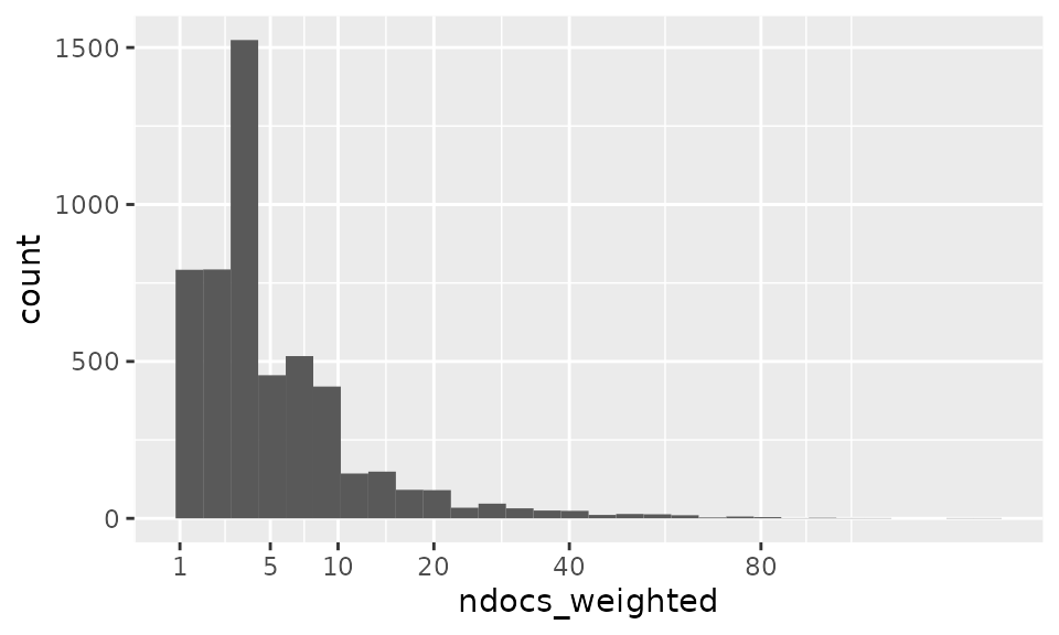

Example: authors with the most documents

The table calculated above makes it possible to assess which authors are represented the most in the corpus.

tib %>% 
  arrange(desc(ndocs_weighted)) %>% 
  head(10)
#> # A tibble: 10 × 3
#>    AU            ndocs_weighted ndocs
#>    <chr>                  <int> <int>
#>  1 PIEGAY H                 142    51
#>  2 RADAKOVITCH O            134    29
#>  3 RABOUILLE C              108    23
#>  4 MARMONIER P              107    37
#>  5 GREMARE A                 95    15
#>  6 OLIVIER JM                93    22
#>  7 GARCIA F                  86     4
#>  8 RAIMBAULT P               84    16
#>  9 BERNE S                   83    14
#> 10 HEUSSNER S                80    17

Table tib_doc_keyword

The table produced by bib_tib_doc_keyword() is structured as **one row = one document*keyword**.

tib_doc_keyword=bib_tib_doc_keyword(tib_doc)

Most frequent keywords

This table can be used to produce a table and graphic showing the most frequently used keywords

tib=tib_doc_keyword %>% 
  group_by(DE) %>% 
  summarise(n=n()) %>% 
  arrange(desc(n)) %>% 
  slice_max(n,n=20)
tib
#> # A tibble: 20 × 2
#>    DE                     n
#>    <chr>              <int>
#>  1 RHONE RIVER          151
#>  2 MEDITERRANEAN SEA     72
#>  3 FRANCE                59
#>  4 GULF OF LIONS         54
#>  5 RHONE                 54
#>  6 MEDITERRANEAN         49
#>  7 SEDIMENT              48
#>  8 RIVER                 43
#>  9 CLIMATE CHANGE        35
#> 10 FISH                  35
#> 11 DISTURBANCE           28
#> 12 HOLOCENE              28
#> 13 ORGANIC MATTER        26
#> 14 MACROINVERTEBRATES    25
#> 15 SEDIMENTS             24
#> 16 FLOODPLAIN            23
#> 17 FLOODS                21
#> 18 SEDIMENT TRANSPORT    21
#> 19 CONNECTIVITY          20
#> 20 GULF OF LION          19

The most frequent keywords can then be displayed as a graphic either directly through a ggplot2 plot or using package https://github.com/lvaudor/mixr.

mixr::plot_frequencies(tib,cat=DE,frequency=n,fill_fixed="dark blue")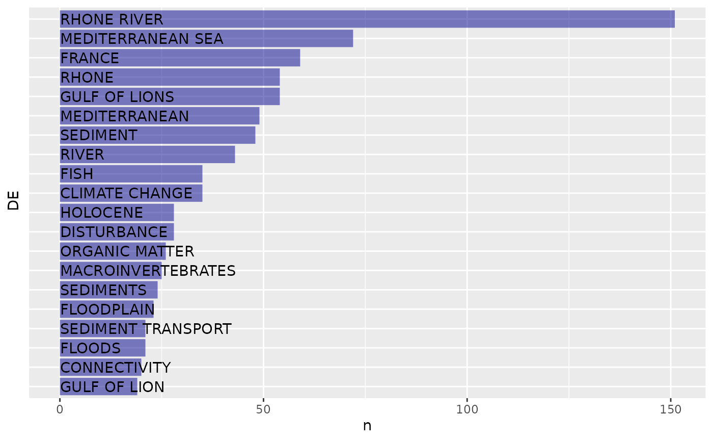

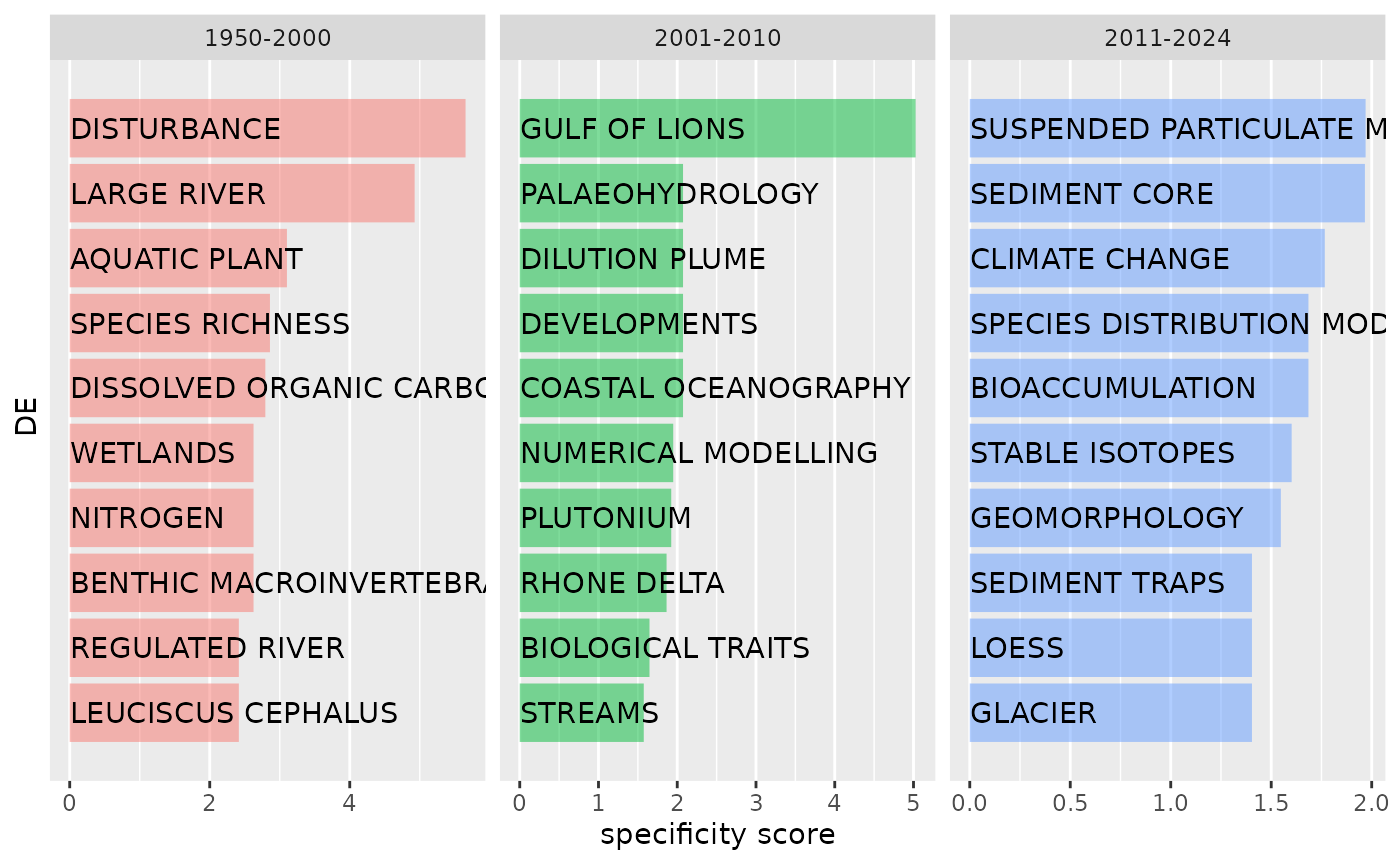
Keywords specific to a part of the corpus

One can also analyse the keywords which are specific to certain parts of the corpus. Let’s divide our present corpus into two parts, based on publication date:

tib_doc_keyword=tib_doc_keyword %>% 
  mutate(period=cut(PY,breaks=c(1950,2000,2010,2024),
                    labels=c("1950-2000","2001-2010","2011-2024")))

We will use package https://github.com/lvaudor/mixr to calculate specificity scores of keywords regarding these periods.

df_spec=mixr::tidy_specificities(tib_doc_keyword,cat1=DE,cat2=period,top_spec=10)
mixr::plot_specificities(df_spec,DE,period)